Activating neurons with Gated Linear Units (GLU) and Friends

Activation functions are a crucial component of every neural network. They introduce non-linearity to the model, allowing it to learn complex patterns in the data.

The chain of operations in a 2-layer neural network can be formulated as follows:

where \(g\) is the activation function, \(W_1\) and \(W_2\) are the weight matrices, \(b_1\) and \(b_2\) are the bias vectors, and \(x\) is the input vector.

So what would happen if we used a linear activation function \(g(x) = x\)?

We would end up with a linear model, which is not very useful for learning complex mappings.

In this post, we will explore activation functions derived from the Gated Linear Unit (GLU) as introduced in Shazeer et al. (2020), and their effectiveness in learning a task when applied to the feed-forward module in the Transformer architecture.

Introduction

The Transformer model processes the input data by alternating between multi-head attention and “point-wise feed-forward networks” (FFN). In its basic form, the FFN is typically applied on each input token independently, and consists of two linear layers with a non-linear activation function in between.

Glorot et al. (2011) introduced the Rectified Linear Unit (ReLU) activation function, which has become a popular choice in deep learning models. The ReLU function is defined as:

Or as applied to the FFN:

Hendrycks and Gimpel (2016) suggested replacing ReLU with the Gaussian Error Linear Unit, or GELU, activation function:

where \(\Phi\) is the cumulative distribution function of the standard normal distribution, and \(\text{erf}\) is the error function. It is possible to approximate the GELU function with the following expression:

When applied to the FFN, we obtain:

Ramachandran et al. (2017) introduced by the Swish activation function:

When \(\beta = 1\), the function becomes equivalent to the Sigmoid Linear Unit (Elfwing et al., 2017), or SiLU:

When applied to the FFN, we obtain:

where we assume \(\beta = 1\) for simplicity.

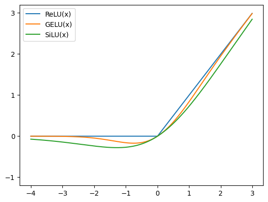
Above we can see the plots of the activation functions discussed in this section.

Gated Linear Units (GLU) and Variants

Dauphin et al. (2016) introduced the Gated Linear Unit (GLU) activation function, which is defined as the element-wise product of two projections of the input, the first of which is passed through a sigmoid function:

Moreover, they also suggest ommiting the sigmoid activation, which they call the “bilinear” layer:

This way, Shazeer et al. (2020) create several variants of the GLU activation function, by combining it with the activation functions introduced earlier:

Using these as a basis, it is possible to create several variations of the FFN module in the Transformer architecture:

where the bias term is ommited for simplicity.

Notice that all of these layers have 3 weight matrices as opposed to the original 2 in the FFN module. Appropriately, the dimensionality of the projections are adjusted to match the total number of parameters in the original FFN module so that a fair comparison can be made.

Experiments

Using the above FFN proposals, Shazeer et al. (2020) conducted experiments in order to evaluate the effectiveness of the different activation functions.

A T5 model is trained on a denoising objective of predicting missing text segments, and subsequently fine-tuned on various language understanding tasks.

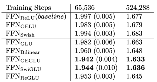
First, they evaluated the log-perplexity by training the model on the C4 dataset, and evaluating it on a held-out validation set. The GEGLU and SwiGLU activation functions outperformed the rest.

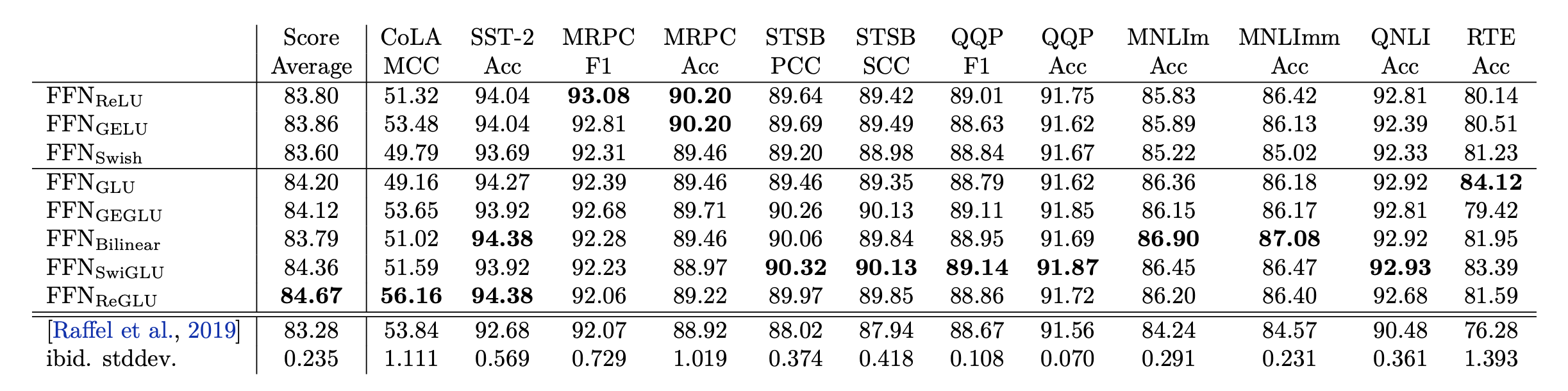
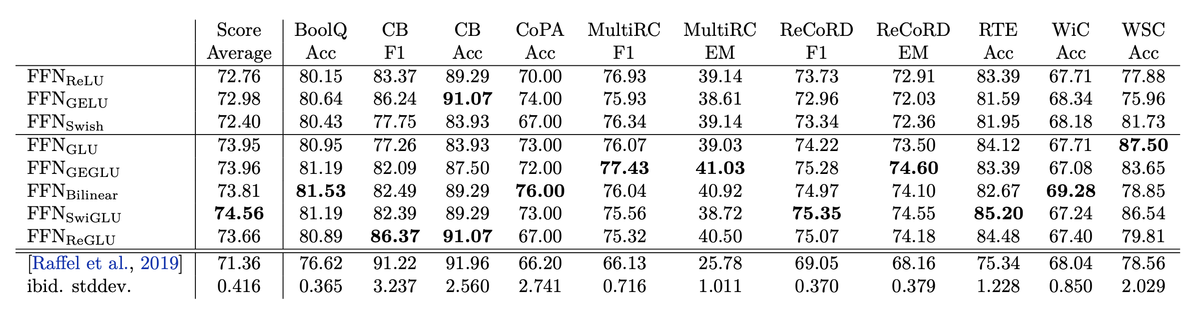
Next, they fine-tune each individual pre-trained model on a set of language understanding tasks from the GLUE and SuperGLUE benchmarks. While the results are noisy, the GLU variants perform best on all of the tasks.

Conclusion

In this post, we have explored several variations of the Gated Linear Unit (GLU) activation function, and their effectiveness in learning a task when applied to the feed-forward module in the Transformer architecture.

The results suggest that the GEGLU and SwiGLU activation functions outperform the rest in terms of log-perplexity on the C4 dataset, and fine-tuning on various language understanding tasks.

So what variation do State-of-the-Art models use today?

Google’s Gemma uses the GEGLU activation function:

class GemmaMLP(nn.Module):
    def __init__(
        self,
        hidden_size: int,
        intermediate_size: int,
        quant: bool,
    ):
        super().__init__()
        self.gate_proj = Linear(hidden_size, intermediate_size, quant)
        self.up_proj = Linear(hidden_size, intermediate_size, quant)
        self.down_proj = Linear(intermediate_size, hidden_size, quant)

    def forward(self, x):
        gate = self.gate_proj(x)
        gate = F.gelu(gate, approximate="tanh")
        up = self.up_proj(x)
        fuse = gate * up
        outputs = self.down_proj(fuse)
        return outputs

Whereas, Meta’s LLaMA uses the SwiGLU activation function:

class FeedForward(nn.Module):
    def __init__(
        self,
        dim: int,
        hidden_dim: int,
        multiple_of: int,
        ffn_dim_multiplier: Optional[float],
    ):
        super().__init__()
        hidden_dim = int(2 * hidden_dim / 3)
        # custom dim factor multiplier
        if ffn_dim_multiplier is not None:
            hidden_dim = int(ffn_dim_multiplier * hidden_dim)
        hidden_dim = multiple_of * ((hidden_dim + multiple_of - 1) // multiple_of)

        self.w1 = ColumnParallelLinear(
            dim, hidden_dim, bias=False, gather_output=False, init_method=lambda x: x
        )
        self.w2 = RowParallelLinear(
            hidden_dim, dim, bias=False, input_is_parallel=True, init_method=lambda x: x
        )
        self.w3 = ColumnParallelLinear(
            dim, hidden_dim, bias=False, gather_output=False, init_method=lambda x: x
        )

    def forward(self, x):
        return self.w2(F.silu(self.w1(x)) * self.w3(x))

Which one is better? Noam puts it best:

“We offer no explanation as to why these architectures seem to work; we attribute their success, as all else, to divine benevolence.”