Stabilizing training and improving model convergence with RMSNorm
In this post, we will discuss RMSNorm, which is a simple and effective method for stabilizing training and boosting model convergence.
This normalization method has been extensively used in various State-of-the-Art transformer models such as LLaMA, Gemma, and Mistral.
Introduction
Deep neural networks have been hypothesized to suffer from the internal covariate shift problem, which occurs when the distribution of the inputs to a layer changes with each training iteration, therefore destabilizing the learning process.
\[ \begin{align} a_i &= \sum_{j=1}^{m} w_{ij} x_j + b_i \\ y_i &= f(a_i) \end{align} \]where \(w_{ij}\) are the weights, \(b_i\) is the bias, and \(f\) is the activation function. This process is repeated for each layer in the network.
Once we make a final prediction, we compute the loss with respect to the ground truth labels, and then backpropagate the gradients to update the model’s parameters.
However, due to the nature of the chain rule, the gradients in the deeper layer get updated first, whereas the gradients in the shallower layers get updated last.
Therefore, the later layers have to constantly adapt to the changing distribution of the input data, since they have not accounted for the (newly introduced) changes in the earlier layers for the next iteration.
\[ \begin{align} \bar{a}_i &= \frac{a_i - \mu_i}{\sigma_i} \cdot \gamma_i + \beta_i \\ \end{align} \]\[ \begin{align} \mu_i = \frac{1}{B} \sum_{b=1}^{B} a_i^{(b)} \quad\quad \sigma_i = \sqrt{\frac{1}{B} \sum_{b=1}^{B} (a_i^{(b)} - \mu_i)^2} \end{align} \]are the mean and standard deviation of the activations across the batch, \(\gamma_i\) and \(\beta_i\) are learnable parameters, and \(B\) is the batch size. This way, the activations are invariant to re-centering and scaling, which makes the model more robust to the changes in the input distribution.
A key drawback of this method is that it introduces a dependency between the features within a batch, which can cause the model to behave unexpectedly during inference, and can even destabilize the training process depending on which items are present in the batch.
\[ \begin{align} \bar{a}_i &= \frac{a_i - \mu_i}{\sigma_i} \cdot \gamma_i + \beta_i \\ \end{align} \]\[ \begin{align} \mu_i = \frac{1}{n} \sum_{j=1}^{n} a_j \quad\quad \sigma_i = \sqrt{\frac{1}{n} \sum_{j=1}^{n} (a_j - \mu_i)^2} \label{eq:layernorm} \end{align} \]Notice that the mean and standard deviation are computed across the features (last dim of the activation tensor) instead of the batch.
RMSNorm
\[ \begin{align} \bar{a}_i &= \frac{a_i}{\text{RMS}(\bf{a})} \cdot \gamma_i \end{align} \]\[ \begin{align} \text{RMS}(\bf{a}) = \sqrt{\frac{1}{n} \sum_{j=1}^{n} a_j^2} \end{align} \]In essence, RMSNorm totally removes the mean statistic in Equation \eqref{eq:layernorm} at the cost of sacrificing re-centering invariance. This vastly simplifies the normalization process, which results in computational gains.
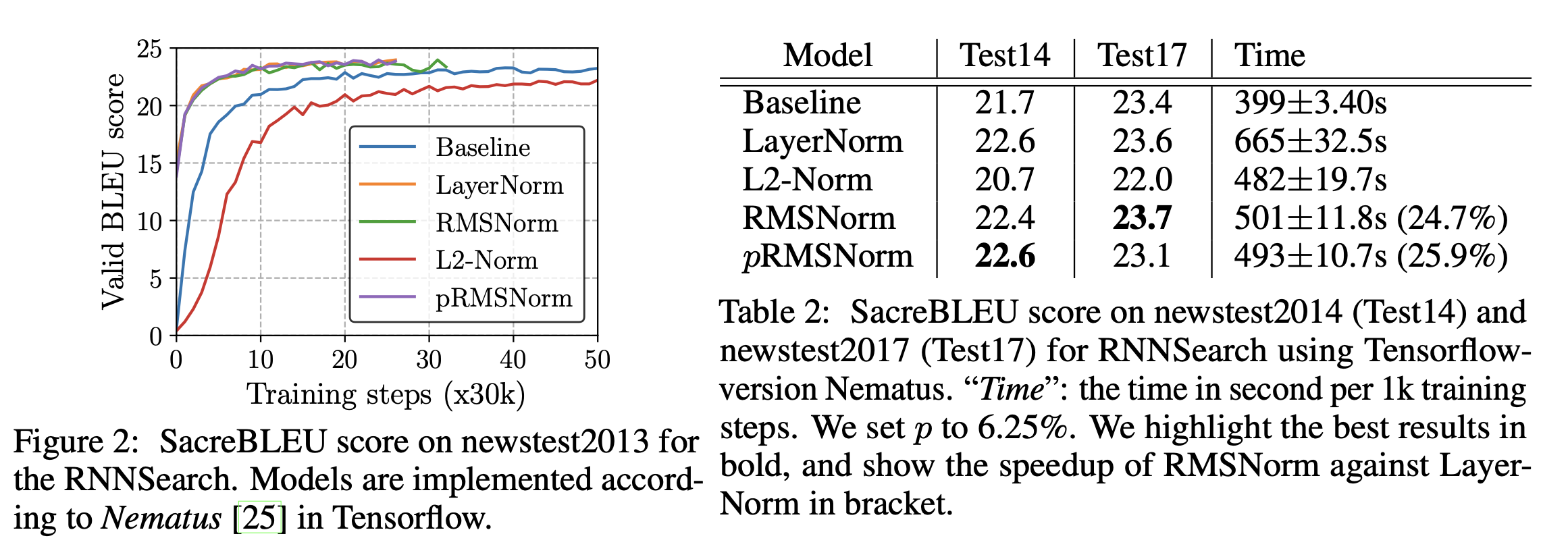
The authors evaluate the performance of RMSNorm, and find that it roughly performs on par with LayerNorm, while being significantly computationally cheaper.
The PyTorch implementation of RMSNorm is relatively straightforward:
class RMSNorm(torch.nn.Module):
    def __init__(self, dim: int, eps: float = 1e-6):
        super().__init__()
        self.eps = eps
        self.weight = nn.Parameter(torch.ones(dim)) # the learnable gamma parameter

    def _norm(self, x):
        return x * torch.rsqrt(x.pow(2).mean(-1, keepdim=True) + self.eps)

    def forward(self, x):
        output = self._norm(x.float()).type_as(x)
        return output * self.weight
Conclusion
In this post, we discussed RMSNorm, a simple and effective method for stabilizing training and boosting model convergence. We compared it to BatchNorm and LayerNorm, and showed that it performs on par with LayerNorm while being significantly computationally cheaper.