Decoupling weight decay with AdamW

13.07.2024 22:58

In this blog we are going to explore how AdamW improves upon the standard Adam optimizer by decoupling the weight decay from the optimization step.

If readers are familiar with the background of Adam, they can skip to the section on AdamW.

Adam

Gradient Descent is a popular optimization algorithm used when the optimum cannot be calculated in closed form. Typically, the learning alorithm can be summarized as follows:

Initialize the weights $w^0$ and pick a learning rate $\alpha$.
For all data points $i \in \{ 1, \ldots, N\} $: forward propagate $x_i$ through the network to get the prediction $\hat{y}_i$, and compute the loss $\mathcal{L}_i(\hat{y}_i, y_i, w^t)$.
Update the weights: $w^{t+1} = w^t - \alpha \frac{1}{N}\sum_{i=1}^N \nabla_w \mathcal{L}_i \left(w^t\right) $.
If the validation error continues to decrease, go to step 2, otherwise stop.

Since pure Gradient Descent requires calculating the gradient for each data point in the dataset before taking even a single step, it can be slow to converge.

To speed up the learning process, Stochastic Gradient Descent (SGD) was introduced. SGD instead computes the gradient for a small random batch of data points, and updates the weights based on this mini-batch. The goal is to approximate the true gradient by using a mini-batch of data points:

\[ \frac{1}{N}\sum_{i=1}^N \nabla_w \mathcal{L}_i \left(w^t\right) \approx \frac{1}{B}\sum_{b=1}^B \nabla_w \mathcal{L}_b \left(w^t\right) \]

such that $B \ll N $.

But even SGD is not perfect, since it scales the gradient equally in all directions. This can lead to slow convergence as highly oscilating gradient directions will slow down the learning process. A potential solution would focus on dampening the directions which oscillate the most, and amplify the directions which are stable across different batches.

In order to tackle this issue, two solutions have been proposed:

SGD with Momentum (Sutskerver et al., 2013) computes a moving average of the gradients, which helps to dampen the oscillations: \[ \begin{align*} m^{t+1} &= \beta_1 m^t + (1-\beta_1) \nabla_w \mathcal{L}_i \left(w^t\right) \\ w^{t+1} &= w^t - \alpha \cdot m^{t+1} \end{align*} \]
RMSProp (Tieleman and Hinton, 2012) scales the learning rate for each parameter by dividing it with the variance of the gradients: \[ \begin{align*} v^{t+1} &= \beta_2 v^t + (1-\beta_2) \left(\nabla_w \mathcal{L}_i \left(w^t\right) \nabla_w \odot \mathcal{L}_i \left(w^t\right) \right) \\ w^{t+1} &= w^t - \alpha \cdot \frac{\nabla_w \mathcal{L}_i \left(w^t\right)}{\sqrt{v^{t+1} + \epsilon}} \end{align*} \] where $\odot$ denotes the element-wise (Hadamard) product, and $\epsilon$ is a small constant to avoid division by zero.

With that said, Adam combines the benefits of both SGD with Momentum and RMSProp. It computes the moving average of the gradients and scales the learning rate for each parameter by dividing it with the variance of the gradients. The update rule for Adam is as follows:

One caveat is that we have to perform bias correction for the moving averages, as they are initialized to zero.

In order to derive the bias correction term, let us first notice how we can re-write the momentum update term (with the same following for the variance term). First, let us denote:

\[ \begin{align*} g_t &= \nabla_w \mathcal{L} \left(w^t\right) &\text{(rewrite for better readibility)}\\ m^0 &= 0 &\text{(initialize momentum to zero)} \end{align*} \]

Then, let us expand the momentum update term:

\[ \begin{align*} m^1 &= \beta_1 m^0 + (1-\beta_1) g_0 \\ &= (1-\beta_1) g_0 \\ m^2 &= \beta_1 m^1 + (1-\beta_1) g_1 \\ &= \beta_1 (1-\beta_1) g_0 + (1-\beta_1) g_1 \\ m^3 &= \beta_1 m^2 + (1-\beta_1) g_2 \\ &= \beta_1^2 (1-\beta_1) g_0 + \beta_1 (1-\beta_1) g_1 + (1-\beta_1) g_2 \\ \implies m^t &= (1-\beta_1) \sum_{i=0}^{t-1} \beta_1^{t-1-i} g_i \end{align*} \]

Therefore, the expectation over the momentum term is:

\[ \begin{align*} \mathbb{E} \left[m^t \right] &= \mathbb{E} \left[ (1-\beta_1) \sum_{i=0}^{t-1} \beta_1^{t-1-i} g_i \right] \\ &= (1-\beta_1) \sum_{i=0}^{t-1} \beta_1^{t-1-i} \mathbb{E} \left[ g_i \right] \\ &\approx \mathbb{E}\left[g_t \right] (1-\beta_1) \sum_{i=0}^{t-1} \beta_1^{t-1-i} \\ &= \mathbb{E}\left[g_t \right] (1-\beta_1) \sum_{i=0}^{t-1} \beta_1^{i} \\ &= \mathbb{E}\left[g_t \right] (1-\beta_1) \frac{1-\beta_1^t}{1-\beta_1} &\text{(geometric series sum)} \\ &= \mathbb{E}\left[g_t \right] (1-\beta_1^t) \end{align*} \]

Reminder that the geometric series sum is calculated as follows:

\[ \begin{align*} s_n &= ar^0 + ar^1 + ar^2 + \ldots + ar^{n-1} \\ &= \sum_{i=0}^{n-1} ar^i \\ &= \cases{a \frac{1-r^n}{1-r} & $r \neq 1$ \\ na & $r = 1$} \end{align*} \]

such that in our case $ a=1$ and $r=\beta_1 \neq 1 $.

With this in mind, for the bias-corrected momentum update we have:

\[ \begin{align*} \hat{m}^t &= \frac{m^t}{1-\beta_1^t} \end{align*} \]

Analogously, we can derive the bias correction term for the variance update:

\[ \begin{align*} \hat{v}^t &= \frac{v^t}{1-\beta_2^t} \end{align*} \]

Putting everything together, we get:

\[ \begin{align*} m^{t+1} &= \beta_1 m^t + (1-\beta_1) \nabla_w \mathcal{L}_i \left(w^t\right) &\text{(SGD with Momentum)} \\ v^{t+1} &= \beta_2 v^t + (1-\beta_2) \left(\nabla_w \mathcal{L}_i \left(w^t\right) \nabla_w \odot \mathcal{L}_i \left(w^t\right) \right) &\text{(RMSProp)} \\ \hat{m}^{t+1} &= \frac{m^{t+1}}{1-\beta_1^{t+1}} &\text{(bias correction for momentum)} \\ \hat{v}^{t+1} &= \frac{v^{t+1}}{1-\beta_2^{t+1}} &\text{(bias correction for variance)} \\ w^{t+1} &= w^t - \alpha \cdot \frac{\hat{m}^{t+1}}{\sqrt{\hat{v}^{t+1} + \epsilon}} \end{align*} \]

AdamW

AdamW is a variant of Adam that decouples weight decay from the optimization step.

As introduced in Hanson & Pratt (1988), weight decay is a regularization technique which decays the weights exponentially during the update steps:

\[ w^{t+1} = (1-\lambda) w^t - \alpha \nabla_w \mathcal{L} \left( w^t \right) \]

where $\lambda $ defines the rate of weight decay per step.

Interestingly, in standard SGD, weight decay is equivalent to adding the L2 regularization term $\frac{\lambda'}{2} \Vert w \Vert_2^2 $ to the optimization objective, where $\lambda' = \frac{\lambda}{\alpha}$.

Consider the following (total) loss function:

\[ \mathcal{L}_{\text{total}} = \mathcal{L}(w) + \frac{\lambda'}{2} \Vert w \Vert_2^2 \]

Then, the gradient of the total loss function is:

\[ g_t = \nabla_w \mathcal{L}_{\text{total}} = \nabla_w \mathcal{L}(w) + \lambda' w \]

Therefore, during the update step we have

\[ \begin{align*} w^{t+1} &= w^t - \alpha \nabla_w \mathcal{L}_{\text{total}} \left( w^t \right) \\ &= w^t - \alpha \left( \nabla_w \mathcal{L}(w^t) + \lambda' w^t \right) \\ &= w^t - \alpha \nabla_w \mathcal{L}(w^t) - \alpha \frac{\lambda}{\alpha} w^t \\ &= (1-\lambda) w^t - \alpha \nabla_w \mathcal{L}(w^t) \end{align*} \]

Whereby we obtain the equivalence between $L_2$ regularization and weight decay. Typically, deep learning frameworks implement $L_2$ regularization by modifying the gradient of the original loss function with $\lambda' w$:

\[ g_t = \nabla_w \mathcal{L}(w) + \lambda' w \]

where $\lambda' = \frac{\lambda}{\alpha}$ is coupling the learning rate $\alpha$ with the weight decay rate $\lambda$.

However, the equivalence between $L_2$ regularization and weight decay does not hold for adaptive gradient methods!

Let us consider the update step for SGD with Momentum:

\[ \begin{align*} m^{t+1} &= \beta_1 m^t + (1-\beta_1) \nabla_w \mathcal{L}_{\text{total}} \left( w^t \right) \\ &= \beta_1 m^t + (1-\beta_1) \left( \nabla_w \mathcal{L}(w^t) + \lambda' w^t \right) \\ &= \beta_1 m^t + (1-\beta_1) \nabla_w \mathcal{L}(w^t) + (1-\beta_1) \frac{\lambda}{\alpha} w^t \\ \\ w^{t+1} &= w^t - \alpha m^{t+1} \\ &= w^t - \alpha \left( \beta_1 m^t + (1-\beta_1) \nabla_w \mathcal{L}(w^t) + (1-\beta_1) \frac{\lambda}{\alpha} w^t \right) \\ &= w^t -\alpha \left( \beta_1 m^t + (1-\beta_1) \nabla_w \mathcal{L}(w^t) \right) - (1-\beta_1) \lambda w^t \\ &= (1 - \underbrace{(1-\beta_1)}_{\text{extra factor}} \lambda) w^t - \alpha \left( \beta_1 m^t + (1-\beta_1) \nabla_w \mathcal{L}(w^t) \right) \end{align*} \]

As we see, we get an extra (unexpected) factor $(1-\beta_1)$, which makes it inequivalent to the pure weight decay form. The same holds for Adam, which also experiences this for the variance update term.

In order to both: 1) decouple the $(1-\beta)$ term from the weight decay $\lambda$, and 2) decouple the learning rate $\alpha$ from the weight decay rate $\lambda$ introduced in $\lambda'$, AdamW simplifies the learning process by leaving the gradients unmodified, and instead adding the weight decay term directly to the update step:

where $\lambda$ is not coupled with the learning rate $\alpha$.

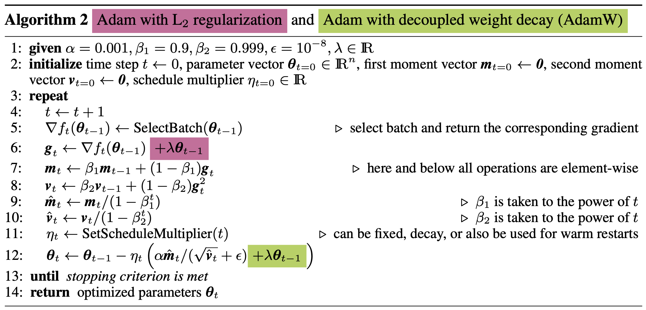
Above is the full AdamW algorithm as layed out in the paper. Notice that the method also has a schedule multiplier factor $\eta_t$ in order to allow for possible scheduling of both $\alpha$ and $\lambda$.