Encoding positional information with Rotary Position Embeddings (RoPE)

Rotary Position Embeddings (RoPE) is a position encoding method which has found its way in several popular transformer architectures: LLaMA 3, Gemma, GPT-J and many more.

Here is a short summary from the abstract of the paper:

“The proposed RoPE encodes the absolute position with a rotation matrix and meanwhile incorporates the explicit relative position dependency in self-attention formulation. Notably, RoPE enables valuable properties, including the flexibility of sequence length, decaying inter-token dependency with increasing relative distances, and the capability of equipping the linear self-attention with relative position encoding.”

In this post, I provide a brief overview of RoPE and the motivation behind it.

We will first start off with how other positional encoding methods work. Next, we provide the necessary background and derivation of RoPE. Finally, we will take a step back and discuss the high-level intuition behind RoPE and why it seems to work so well in practice.

Related Work

Let \( \mathbb{S}_N = \{ w_i \}_{i=1}^N \) be a sequence of \(N\) input tokens with \(w_i\) being the \(i\)-th token. The corresponding word embedding of \(\mathbb{S}_N \) is denoted as \(\mathbb{E}_N = \{ \bf{x}_i\}_{i=1}^N \), where \(\bf{x}_i \in \mathbb{R}^d \) is the \(d\)-dimensional embedding of \(w_i\) without position information.

Self-attention first incorporates position information to the word embeddings and transforms them into queries, keys, and values:

where \( \bf{q}_m\), \(\bf{k}_n\) and \(\bf{v}_n\) incorporate the \(m\)-th and \(n\)-th positions through \(f_q\), \(f_k\) and \(f_v\) respectively. The query and key values are then used to compute the attention weights, while the output is computed as the weighted sum over the values:

Most approaches to positional encoding can be grouped in two categories: absolute and relative.

Absolute position embedding

A typical choice for the function \(f\) is:

where \( \bf{p}_i \) is a \(d\)-dimensional positional encoding vector.

Previous work Devlin et al. (2019), Lan et al. (2020), Clark et al. (2020), Radford et al. (2019), Radford and Narasimhan (2018) introduced the use of a set of trainable vectors \( \bf{p}_i \in \{ \bf{p}_t \}_{t=1}^L\), where \(L\) is the maximum sequence length.

The authors of Vaswani et al. (2017) have proposed to generate \(\bf{p}_i\) using the sinusoidal function:

in which \(\bf{p}_{i, 2t}\) is the \(2t\)-th element of the \(d\)-dimensional vector \(\bf{p}_i\).

Relative position embedding

The authors of Shaw et al. [2018] parametrize \(f\) as follows:

where \(\tilde{\bf{p}}_r^k\) and \(\tilde{\bf{p}}_r^v\) are trainable relative position embeddings. Note that \(r = \text{clip} (m-n, r_{\text{min}}, r_{\text{max}})\) represents the relative distance between position \(m\) and \(n\). The clipping is done under the hypothesis that precise relative position information is not useful beyond a certain distance.

Dai et al. (2019) have proposed to decompose \(\bf{q}_m^T \bf{k}_n\) of Equation \eqref{eq:attention} as follows:

with the proposed change to replace the absolute position embedding \(\bf{p}_n\) with its sinusoid-encoded relative counterpart \(\tilde{\bf{p}}_{m-n}\), while the absolute position \(\bf{p}_m\) in the third and fourht term with two trainable vectors \(\bf{u}\) and \(\bf{v}\) independent of the query positions. Further, \(\bf{W}_k\) is distinguished for the content-based and location-based key vectors \(\bf{x}_n\) and \(\tilde{\bf{p}}_{m-n}\), denoted as \(\bf{W}_k\) and \(\tilde{\bf{W}}_k\), resulting in:

There are several other variations, but we live it to the reader to explore them further.

Theoretical Explanation of RoPE

Transformers natively don’t incorporate positional information, hence the need to incorporate it through positional encodings. The self-attention mechanism outlined in Equation \eqref{eq:attention} enables propagating knowledge between tokens at different positions via \( \bf{q}_m^T \bf{k}_n \). In order to incorporate relative positional information, the authors of RoPE precisely focus on this dot product, with the goal of deriving a function \(g\) which takes as inputs the word embeddings \(\bf{x}_m\), \(\bf{x}_n\) and their relative position \(m-n\) as input variables:

and outputs a dot product which incorporates both the content-based and location-based information.

Complex numbers

Before we dive into the derivation of RoPE, let’s first introduce complex numbers and their properties.

A complex number is a number that can be expressed in the form \(a + bi\), where \(a\) and \(b\) are real numbers, and \(i\) is the imaginary unit. The imaginary unit satisfies the property \(i^2 = -1\).

Complex numbers can be represented in several forms:

1. Rectangular (Cartesian) form: \(z = a + bi\), where \(a\) is the real part and \(b\) is the imaginary part.
2. Polar form: \(z = r (\cos \theta + i \sin \theta)\), where \(r\) is the magnitude and \(\theta\) is the angle.
3. Exponential form: \(z = r e^{i \theta}\), where \(r\) is the magnitude and \(\theta\) is the angle. This form is directly related to the polar form due to Euler’s formula: \(e^{i \theta} = \cos \theta + i \sin \theta\).

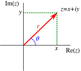
A complex number can visually be represented as a vector in the complex plane, where the real part is the x-coordinate and the imaginary part is the y-coordinate. Conversly, in the polar form, the magnitude of a complex number is the distance from the origin to the point in the complex plane, while the angle is the angle between the positive x-axis and the vector.

Since all forms are equivallent, we can easily convert between them:

1. To go from rectangular to polar form: \[ \begin{align*} r &= \sqrt{a^2 + b^2} \\ \theta &= \arctan \left( \frac{b}{a} \right) \\ z &= r (\cos \theta + i \sin \theta) \end{align*} \]
2. To go from the polar to the exponential form, we can directly utilize Euler’s formula: \[ \begin{align*} z &= r (cos \theta + i \sin \theta) = r e^{i \theta} \end{align*} \]

The neat thing about the exponential form is that rotations are represented simply as multiplication by a complex number. Suppose we have a complex number \(z = r e^{i \theta}\) and we want to rotate it by an angle \(\phi\). We can simply multiply it by \(e^{i \phi}\) to obtain the rotated complex number:

Note that the magnitude is left unchanged because the magnitude of \(e^{i\phi}\) is 1:

This is going to be crucial for the derivation of RoPE.

Derivation of RoPE

First, we consider the case when the embeddings are two-dimensional, i.e. \(d=2\), and later provide a generalized form of the RoPE for higher dimensions.

Consider two word embeddings \(\bf{x}_q\) and \(\bf{x}_k\) which correspond to a query and a key at positions \(m\) and \(n\) respectively. In this case, their position, encoded counterparts are:

where the subscripts of \(\bf{q}_m\) and \(\bf{k}_n\) denote the encoded positional information.

Let us assume that there exists a function \(g\) that defines the inner product between vectors produced by \(f_{\{q, k\}}\):

Furthermore, we require the below initial conditions to be satisfied:

which can be read as the vectors with empty position information encoded.

Given these settings, the authors of RoPE aim to find a solution to \(f_q\) and \(f_k\).

As we disussed earlier, 2D vectors can be interpreted as complex numbers. Therefore, we take advantage of this geometric meaning of a vector in 2D and its complement counter-part, and rewrite the form of \(f_q\), \(f_k\) and \(g\) in terms of complex numbers:

where \(R_q\), \(R_k\) and \(R_g\) are the magnitudes of the vectors, while \(\Theta_q\), \(\Theta_k\) and \(\Theta_g\) are the angles. Plugging these into Equation \eqref{eq:g_inner_product}, we obtain the relation:

Note: Since we are operating in the complex space, the inner product involves complex conjugation, which is the reason why the angles are subtracted.

On the other hand, the initial conditions can be represented as:

where \(\Vert \bf{q} \Vert\), \(\Vert \bf{k} \Vert\) and \(\Theta_q\), \(\Theta_k\) are the magnitudes and angles of the vectors \(\bf{q}\) and \(\bf{k}\) respectively.

Next, we set \(m=n\) in Equation \eqref{eq:rope_magnitude_relation} and take into account the initial conditions to obtain the following relations:

Analogously, when we set \(m=n=0\) in Equation \eqref{eq:rope_angle_relation}, we obtain:

Notice that we get a straight-forward solution for \(R_f\):

which can be interpreted as the radial functions \(R_q\), \(R_k\) and \(R_g\) are independent from the positional information.

On the other hand, for the angular functions we get:

which implies that the angular functions do not depend on the contents of the query and key vectors, but rather on the position of the tokens. Therefore, we can set the angular components in the initial conditions as the same:

As we discussed earlier, the term \(\Theta_f(\bf{x}_{\{q, k\}}, m) - \Theta_{\{q, k\}}\) is a function of the position \(m\) and is independent of the word embedding \(\bf{x}_{\{q, k\}}\). Therefore, we denote this term as:

Now, by plugging \(n=m+1\) to Equation \eqref{eq:rope_angle_relation}, and considering the above relation, we obtain:

Notice that since the RHS is a constant irrelevant to \(m\), \(\Phi(m)\) with continuous integer inputs produces an arithmetic progression. Therefore, we can write \(\Phi(m)\) as:

where \(\Theta\) is the common difference and \(\gamma\) is the initial term.

To summarize our solutions, we have:

Analogously:

Notice that in the above formulation, the authors slightly abuse the notation by jointly using complex numbers and vectors. Nevertheless, we proceed with this notation as it is more intuitive.

In the initial conditions in Equations \eqref{eq:initial_q_functional} and \eqref{eq:initial_k_functional}, we didn’t impose any constraints to the functional forms of \(f_q\) and \(f_k\) and are left to be chosen freely. In order to be consistent with the related work discussed above, the authors of RoPE choose the following functional forms:

where \(\bf{W}_q\), \(\bf{W}_k\) are the trainable projection matrices used in the self-attention mechanism.

Finally, we are also free to set \(\gamma = 0\), and obtain the solutions for \(f_q\) and \(f_k\) as:

As we saw earlier, multiplying a complex number by \(e^{i \theta}\) rotates it by an angle \(\theta\). Therefore, we can further rewrite \(f_{\{q, k\}}\) in matrix-multiplication form:

Therefore, incorporating relative positional embeddings is straightforward:

Simply rotate the affine-transformed word embedding vector by amount of angle multiples proportional to its position index.

General form

In the previous section, we assumed that \(d=2\). In order to generalize our results to any \(\bf{x}_i \in \mathbb{R}^d\) where \(d\) is even, we divide the \(d\)-dimension space into \(d/2\) and combine the results of each two-dimensional case as follows:

where

is the rotary matrix with pre-defined parameters:

Therefore, applying RoPE to the self-attention mechanism yields:

where \( \bf{R}_{\Theta, n-m}^d = (\bf{R}_{\Theta, m}^d)^T \bf{R}_{\Theta, n}^d \).

To understand why the equality of the rotary matrices holds, remember that any rotation matrix \(\bf{R}\) is an orthogonal matrix, therefore \(\bf{R}^T = \bf{R}^{-1}\).

Therefore, the chain of rotations \( (\bf{R}_{\Theta, m}^d)^{T} \bf{R}_{\Theta, n}^d = (\bf{R}_{\Theta, m}^d)^{-1} \bf{R}_{\Theta, n}^d \) can be read as: first go from the n “steps” counter clockwise, and then go back m “steps” clockwise. This is eqivalent to going \((n-m)\) steps counter clockwise, i.e. \(\bf{R}_{\Theta, n-m}^d\)

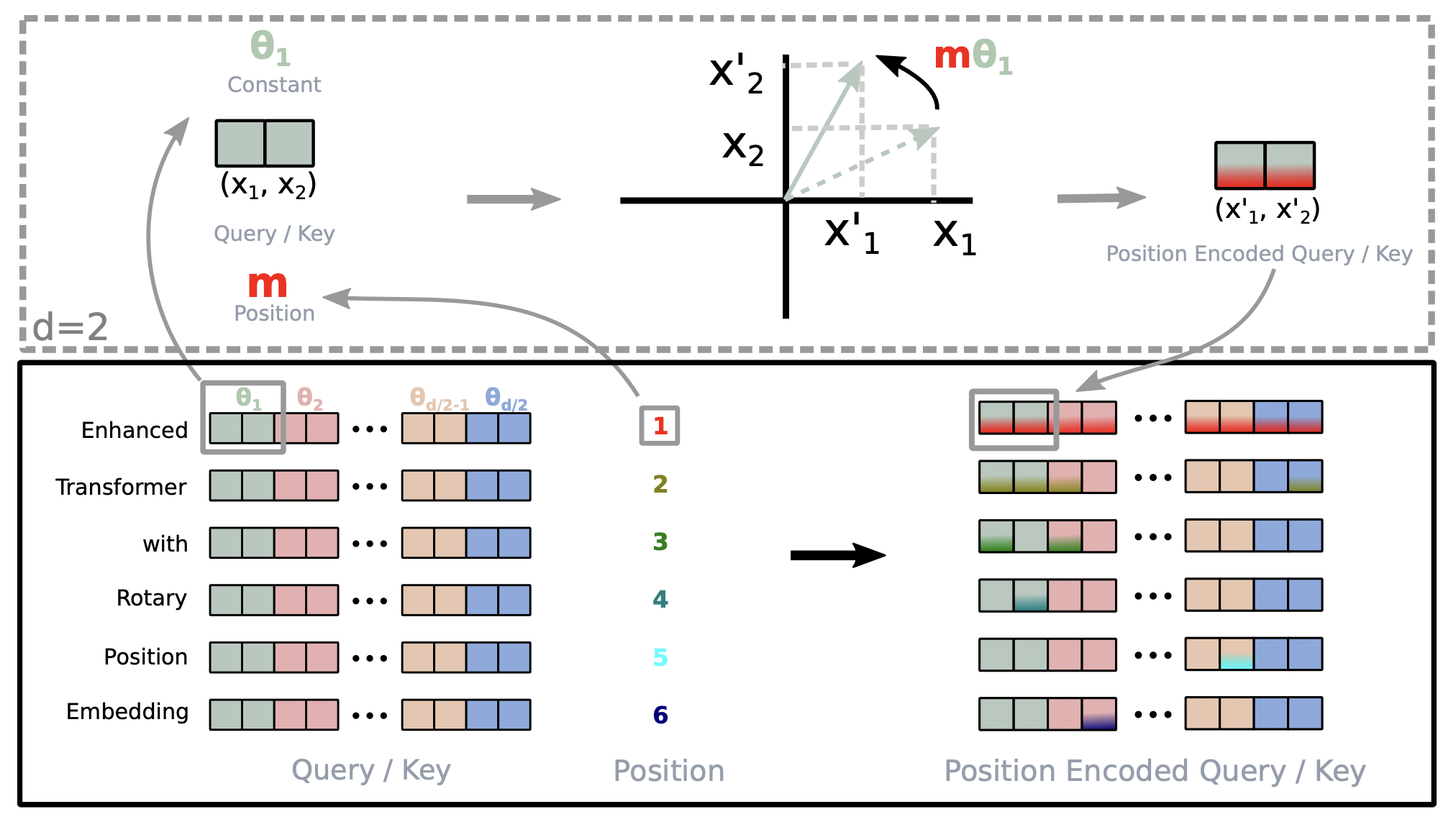
Above is a visual representation of RoPE (source: original paper).

Efficient computation

Note that since the rotation matrix \(\bf{R}_{\Theta, n-m}^d\) is sparse, it is not computationally efficient to perform this matrix multiplication directly.

A more computationally efficient realization is:

which only involves two element-wise multiplications and one addition.

Conclusion

In summary:

• RoPE encodes absolute positional information by rotating each token’s embeddings with a position-specific rotation matrix \( \bf{R}_{\Theta, m}^d \), where \(m\) is the token’s position.
• RoPE also encodes relative positional information, naturally derived from the inner products of the rotated embeddings in the self-attention mechanism: \( \bf{q}_m^T \bf{k}_n = \bf{x}_m^T \bf{W}_q^T \bf{R}_{\Theta, n-m}^d \bf{W}_k \bf{x}_n \).

Appendix

Visualization of RoPE

In this section, we provide several visualizations in order to better understand the RoPE mechanism.

First, let us pre-compute the frequencies for several token positions and embedding dimension pairs:

import matplotlib.pyplot as plt
import seaborn as sns
import torch

def precompute_freqs_cis(dim: int, num_tokens: int, theta: float = 10000.0):
    freqs = 1.0 / (theta ** (torch.arange(0, dim, 2)[: (dim // 2)].float() / dim))
    t = torch.arange(num_tokens, device=freqs.device, dtype=torch.float32)
    freqs = torch.outer(t, freqs)
    freqs_cis = torch.polar(torch.ones_like(freqs), freqs)  # complex64
    return freqs_cis

dim = 512
num_tokens = 128
theta = 10000.0
token_idx = 3

freqs_cis = precompute_freqs_cis(dim, num_tokens, theta)
print(f"Shape: {freqs_cis.shape}, Dtype: {freqs_cis.dtype}")
print(f"First 10 elements (in degrees) for freqs at pos {token_idx}:")
print(torch.rad2deg(torch.angle(freqs_cis[token_idx, :]))[:10])

Shape: torch.Size([128, 256]), Dtype: torch.complex64
First 10 elements (in degrees) for freqs at pos 3:
tensor([171.8873, 165.8131, 159.9536, 154.3011, 148.8483, 143.5883, 138.5141,
        133.6192, 128.8973, 124.3423])

Let us peek at all the frequencies of rotations for the token at position 3:

plt.plot(torch.rad2deg(torch.angle(freqs_cis[token_idx, :])).cpu().numpy())
plt.xlabel('Index of pair in embedding dimension')
plt.ylabel('Rotation (degrees)')
plt.title(f'Rotation angles for token {token_idx}')
plt.show()

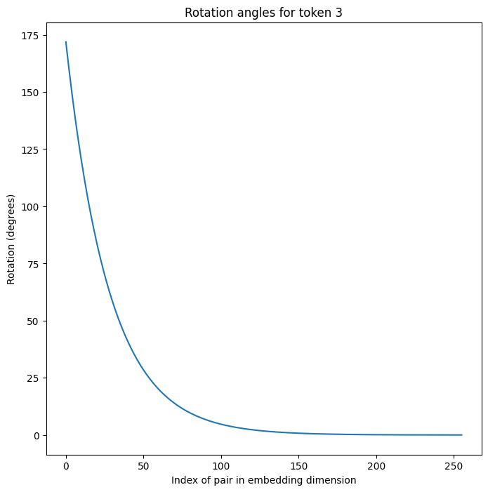
More precisely, in the plot above, we are looking at how much each pair of dimensions is rotated counter-clockwise for the token at position 3.

Therefore, if we rotate a vector whose initial position is \((1, 0)\) using the angles of rotation above:

vec = torch.tensor([1, 0], dtype=torch.float32)
vec_complex = torch.view_as_complex(vec)

freqs_for_token = freqs_cis[token_idx, :]

rotated_vec = vec_complex * freqs_for_token # multiplication in complex space = rotation

plt.figure(figsize=(12, 12))
for i in range(64):
    plt.plot([0, rotated_vec[i].real], [0, rotated_vec[i].imag], color='blue')
    plt.annotate(f'{i+1}', (rotated_vec[i].real, rotated_vec[i].imag), color='red')
plt.plot([0, 1], [0, 0], color='black')
plt.annotate('0', (1, 0), color='red')
plt.axis('equal')
plt.legend()
plt.title(f'Rotated vector at token {token_idx}')
plt.show()

We get the following visualization:

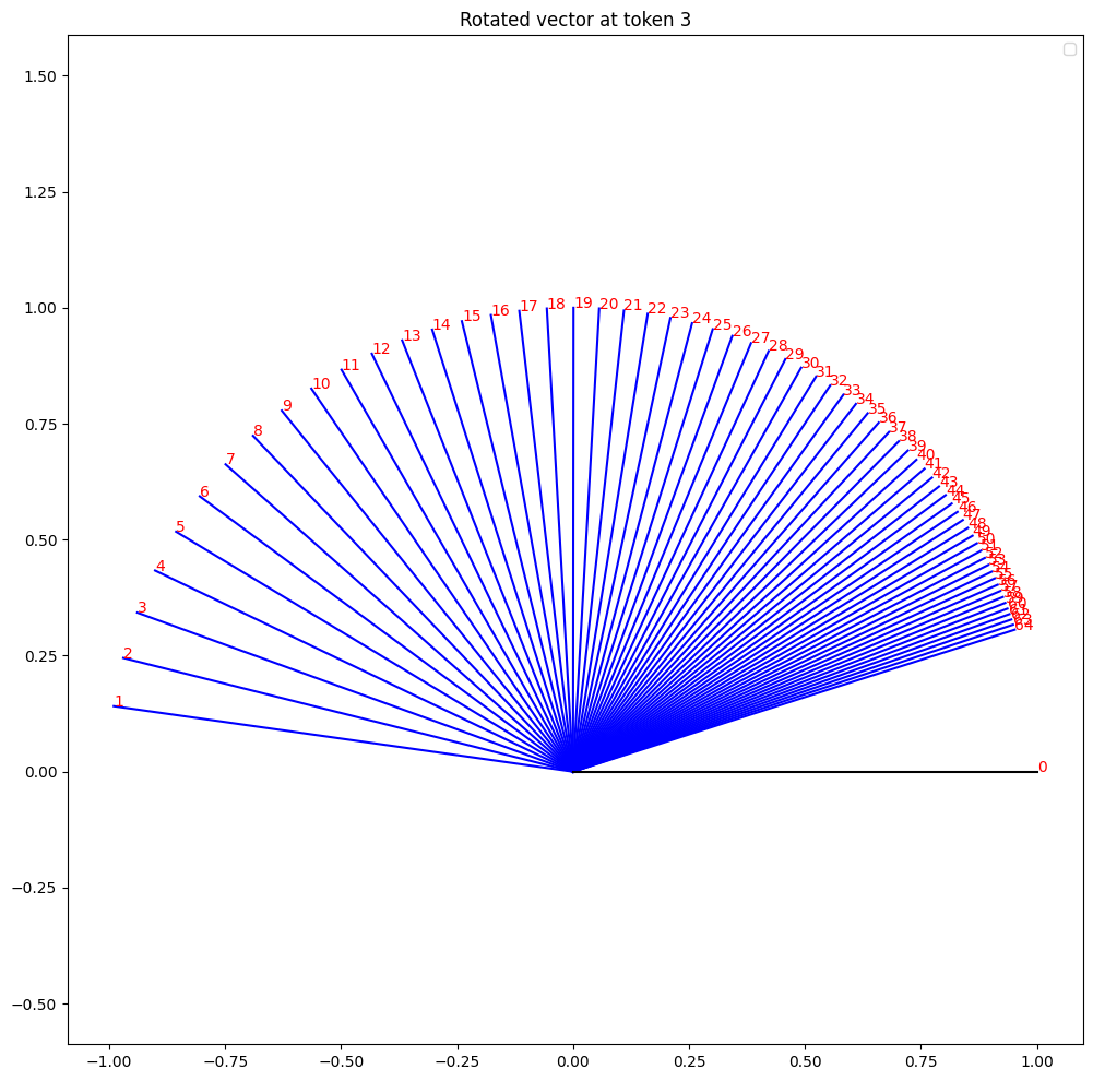
As expected, the initial vector (labeled as 0), is first rotated counter clockwise by an angle of about 171 degrees for the first pair of dimensions, 165 degrees for the second pair, and so on. We don’t show all 256 pairs of dimensions, as they get cluttered, but the pattern is clear.

A question that might arise is:

Are the rotations always monothonic?

No! Let us plot the rotation angles along both the embedding dimensions and the token positions:

plt.figure(figsize=(8, 8))
sns.heatmap(torch.rad2deg(torch.angle(freqs_cis)).cpu().numpy(), cmap='viridis', cbar_kws={'label': 'Rotation Angle (degrees)'})
plt.title('Rotation Angles across Token Positions and Pair Dimensions')
plt.xlabel('Index of pair in embedding dimension')
plt.ylabel('Token Position')
plt.show()

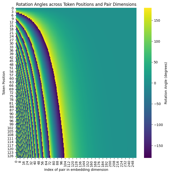
Notice that for many token positions, the rotation angles are not monothonic: they can oscillate between positive and negative values for the angles of rotation.

Extrapolation to longer sequences

Interestingly, it is possible to modify the RoPE mechanism to handle longer sequences than those encountered during training.

Specifically, the mainstream approach to addressing extrapolation with LLMs involves modifying RoPE by replacing \(10000\), the base in \(10000^{-2(i-1)/d}\) in the original formulation with a larger value and providing longer fine-tuning text.

Sometimes, it is possible to even get away without fine-tuning on longer sequences (see here for an exampling involving LLaMA 3).

The main motivation is to spread out the positional embeddings, making them more distinct for longer sequences.